Open Source Air-Bearing Simulation
Janis H. Wortmann, Manuel Scholz
Research and Development
Eitzenberger GmbH Wessobrunn, Bavaria, Germany
ABSTRACT
This paper introduces an open-source air-bearing simulation software written in Python. Using the finite volume method, it solves the Reynolds
Equation over a 2D mesh. It is written modularly, allowing for different sub-models to be used and easily modified by users. Common boundary
conditions such as inlet formulations and basic tools to generate the mesh are provided. The goal is to provide a robust implementation of the methods outlined in the literature for researchers and engineers to use and expand upon.
INTRODUCTION
The analytical and numerical simulation of air bearings has been a field of research for a long time. As such, the history and various methods and approaches are well documented in the literature [1]. However, their implementation requires considerable knowledge of numerical mathematics and coding. Another option is multi- physics software such as COMSOL. It is being used for air-bearing simulation [2] [3]. We found that quite some modeling effort is necessary to achieve good results. Especially for micro-groove and restrictor-regulated bearings and subsequent model fitting, customization is required. While certainly an option to consider for many applications, there are drawbacks to using a small part of a large software suite to analyze a narrowly defined problem. One example is the licensing cost. Combined, there might be a barrier to entry for some and a significant time investment for others to simulate an air bearing. It could be speculated, that considerable duplicative effort has been made to model or write what is essentially the same software, by researchers the world over. The air bearing simulation described here does not claim to be novel in the modeling approach, but rather in the fact that it is an open-source project with accessibility and modularity in mind. Eitzenberger will release the first version of the simulation on Github by the end of 2024, hoping that others will find it helpful, and will consider joining the collaborative development.
MODELLING APPROACH & ARCHITECTURE
For most types of air bearings, the pressure distribution, flow rates, and lift forces are modeled very well by the stationary isothermal Reynolds Equation, which we solve numerically using the finite volume method (FVM) on a triangular mesh. A basic import tool that converts a vector graphic to a suitable mesh (using Gmesh) is provided. An example of such a graphic is shown in Figure 1. It is possible to add an arbitrary number of sub- areas, for which different refinement parameters can be provided. These areas remain labeled after meshing, and as such can then be used to specify height offsets (e.g. for grooves or pockets) or to define inlet/outlet port regions. An example mesh generated from the shown pad design can be seen in Figure 2.
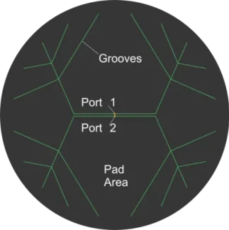
FIGURE 1.
SVG file used to communicate the geometry of the bearing as well as the geometry of sub-areas, such as inlet ports or grooves.
The simulation behavior is governed by a few lightweight module types, that model certain aspects of the physical system. For example, we provide models for constant pressure ports, flow- restricting nozzles, and porous media.
Each of them can be attached to any predefined area on the mesh. Other models control the flow resistance between cells given the gap height or surface velocity-related pressure contributions. Such models can easily be added or modified without changes to the simulation code itself. Given the mesh, the simulation evaluates the attached models and solves for the pressure distribution (Figure 3) under the bearing surface. From this result, several interesting quantities like lift force or flow rates can be extracted and visualized in a post-processing step.
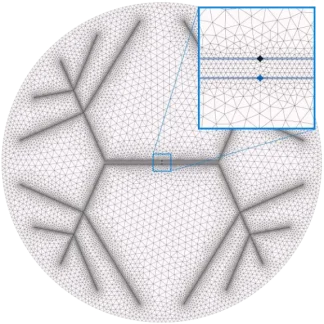
FIGURE 2.
A plot of the 2D mesh with adaptive refinement around predefined areas.
IMPLEMENTATION
Our Python implementation is based on a node- based FVM scheme where control volumes are centered around each node. By limiting ourselves to triangle meshes, it is possible to formulate the pressure gradients as linear combinations of (unknown) node pressures without the need for any approximations or non-orthogonal correctors. The latter can cause severe problems at gap height discontinuities (e.g. groove boundaries) where flow resistance can abruptly vary by orders of magnitude. The formulation used enables us to sidestep these problems altogether. We follow common practice and iteratively linearize the Reynolds equation at the current estimate of the pressure distribution and solve it using a sparse linear solver. Critical code regions are accelerated with a just-in-time compiler (numba library) to maximize performance
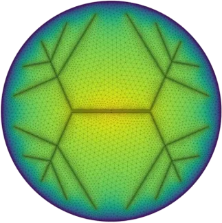
FIGURE 3.
Pressure distribution of an Eitzenberger nozzle and micro-groove regulated air bearing at a given air gap.
DEFINITION OF AIR GAP- WHAT TO VALIDATE AGAINST?
To validate the model, it should be checked against experimental results. To the knowledge of the authors, there is no universal standard to measure the static performance of air bearings. The definition of air gap is not as straightforward as it might seem. One approach, that is often used in manufacturing environments, is to load the bearing as desired. The air supply is then switched off and the displacement measurement between a suitable part of the bearing and the counter surface is zerod. The air supply is then switched on, and the displacement recorded. This displacement is then called ‘air gap’. There are, however, several shortcomings of this approach. Figure 4 shows a selection of the contributors to error. The air bearing might have a concave shape. The planarity of the surfaces is not perfect. The air bearing will deform under pressure. By setting the loaded state to zero, one is blind towards those effects. A better approach is the one used by Vainio et. Al.[5]. Summarizing, they record the system deflection caused by the changing loads in addition to the air on/off data against a suitable setup. That gives an estimation of the possible errors. However, this approach is still blind towards the changing pressure distribution under the bearing causing deflection. The effect can be minimized though, through a sufficiently stiff (validation-) bearing. We found that it is best to first be aware of the possible pitfalls, and then try to minimize them through careful setup design.
While physics doesn’t care whether a particular bit of air gap is caused by concavity, deflection, or the nominal air gap, the distinction is critical when looking at simulated vs. measured lift/load curves. To help with this problem, we suggest to look at the bearing force over the air consumption. Both the force applied to the bearing, and the air consumption of the bearing are less problematic to measure. The model to validate essentially describes the relationship between mass flow and pressure gradients. The air gap influences the flow resistance, with its contribution being notably cubic in nature. Using this method doesn’t substitute building a precision engineered setup, but it is less sensitive to localized errors and focuses more on analyzing the relationship to validate.
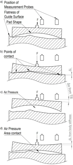
FIGURE 4.
Contributors to error when measuring an air gap.
a): air bearing lightly touching counter surface.
b): air bearing pressed into counter surface. Note the difference in displacement.
c): floating air bearing is less deformed than b). Sensor position also causes a difference.
d): air bearing body deformation due to high force has effect.
Correctly attributing measured air gap to model air gap can be challenging and requires careful setup.
ACCURACY OF RESULTS
With the aforementioned problems in mind, we now present the current state of results for a round pad with 150 mm in diameter that is nozzle and groove regulated. We plotted both the air on / off air gap with constant force and the air on value in reference to 0 force. Figure 5 shows the predicted vs. measured lift-load curves for that bearing.
It has a concavity of 2 um. According to FEM simulations, we expect a reduction of 0.8 um for the concavity depth when considering no load vs. maximum load. Notably, deviations from the measurements are only readily apparent when zoomed in. If we consider a 5 um air gap as an example, the model predicts 6.573 kN of force. Measured with the air off / on method, it takes 6.47 kN or 1.5% less force to reach the air gap. Respectivly, when not considering the deflection due to load, it only takes 6.08 kN to measure 5 um air gap, or 7.5% less. Perhaps less desirable is the position of the stiffness maximum when comparing simulation vs. measurement as seen in Figure 6. While the simulation predicts the stiffness maximum to be at 3.1 um, it is measured to be at 3.5 um or 4.2 um, respectively. From the point of view of an air bearing designer, this is a critical characteristic.
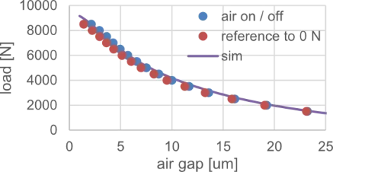
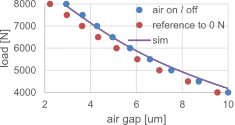
FIGURE 5.
Lift-load curves of D150 validation bearing. Top: total curve. Bottom: zoomed to approximate operating range.
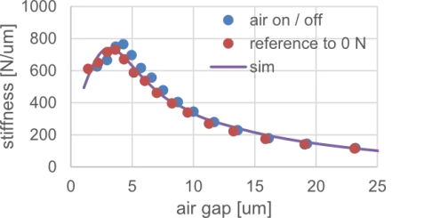
FIGURE 6.
Lift-stiffness curves of D150 validation bearing. Computed as the derivative of the lift- load curve.
As suggested in the last chapter, we will now look at air consumption over load in Figure 7. We included both the nominal 2 um concavity and a 1.2 um variant that represents the calculated change due to loading the air bearing. The curves are very similar, and become more similar with increasing load. We therefore interpret, that the concavity change is not the reason for the error. The model of the validation bearing would likely not considerably benefit from incorporating a fluid-structure interaction. At very low load, the air consumption is a good fit. For the considered bearing type, this region is typically dominated by the inlet nozzles. From an analysis point of view, we interpret this as evidence, that the nozzle model formulation works quite well. In fact, iterating, we could now go back into the simulation and change the nozzle parameters to match the measurements exactly. However, to keep the shown results representative, we refrain from fitting after-the-fact. Then, up to about half load, the error is highest. In this region, flow is also high leading to the result being dominated by large pressure gradients around the nozzle and adjacent grooves. We believe that the underlying assumptions of the Reynolds equation might not be entirely valid here, due to turbulent flow or at least appreciable fluid inertia forces in that specific region. For example, the reynolds number within the groove exceeded 1500, much higher than the usual values in the bearing land, though also lower than the 2300 often used as a tipping point. This might be a conceptual limitation of modeling grooves by using locally increased air gap in the corresponding regions. Attempting to correct for this by changing the flow resistance based on current flow conditions is possible within the simulation. But we still believe it is necessary to emphasize this suspected model limitation. Lastly, in the mid to high load range, the fit is very good. We assume that this is evidence of the general suitability of the chosen modeling approach for the problem at hand.
Given that this load region is of the greatest technical interest, we are satisfied with the current results. Presumably, porous media type bearings might generate even better results, as the model limitations do not apply here. The same should be true for purely nozzle regulated bearings. However, we have not validated these types of bearing yet.
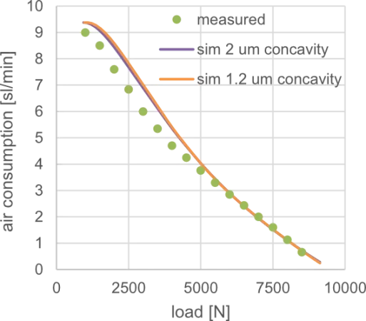
FIGURE 7.
Air consumption over load.
VALIDATION: OPPORTUNITY FOR FUTURE WORK
At this point, there is still more validation work to be done. One idea is to build a set of validation bearings that more heavily utilize certain aspects of the model in their design, compared to other design aspects. For example a bearing that is more nozzle-dependent, or one with an odd shape to emphasize grooves over the area model. Other bearing types would also be interesting. Last but not least, one could also check this model against other numerical models, to check for possible implementation errors.
DYNAMICS: OPPORTUNITY FOR FUTURE WORK
What was presented here is only concerned with the static analysis of air bearings. However, that is only one half of the problem. An air bearing designer is especially concerned with maximizing stiffness, without causing dynamic problems such as low dampening or even air hammer. We are currently considering to implement a pertubation analysis in order to calculate dynamic stiffness and dampening. However, there still is a lot of work to be done. Especially measuring the dynamic characteristics of an air bearing is challenging. It is, however, also necessary in order to validate the model.
SUMMARY
A lightweight air-bearing simulation software was written by implementing methods found in the available literature. It has demonstrated accuracys below 10% in the considererd validation case. It will be made available publicly as an open-source project on the Eitzenberger GitHub page [5].
REFERENCES
[1] Al-Bender, F., Air Bearings: Theory, Design and Applications. John Wiley and Sons, Inc. 2021.
[2] Hwang, P.; Khan, P.; Kang, S.-W. Parameter Sensitivity Analysis on Dynamic Coefficients of Partial Arc Annular-Thrust Aerostatic Porous Journal Bearings. Appl. Sci.
[3] Lentini, L., Colombo, F., Trivella, A., Raparelli, T., & Viktorov, V. Multi-Physical Simulation of Aerostatic Bearings.
[4] Valtteri Vainio, Mikael Miettinen, Jaakko Majuri, René Theska, Raine Viitala. Manufacturing and static performance of porous aerostatic bearings. Precision Engineering. 2023; 84: 177-190.
[5] Eitzenberger GmbH (2024, April 25). Eitzenberger GmbH public GitHub page https://github.com/Eitzenberger-GmbH